Day 8: Simplex optimisation with Perl Data Language

If you want to solve linear programming problems, you need PDL!

This article discusses PDL::Opt::Simplex, and uses PDL::Graphics::Simple to display output.

The simplex algorithm finds the optimum "point" (coordinates) in a space you define, which can have any number (called n here) of dimensions.

The algorithm takes either a fully-formed cloud of n+1 points, or a single starting point, in which case it constructs the cloud for you using the "initsize" parameter. It also takes a function that will take a series of points in your space, and returns the "value" at each of those points. From that, it works out which point of the simplex to move to be closer to the optimum point, which has the lowest value of your function.

It also takes other, less important parameters, which you'll see, including a "logging" function which you can use to report progress, or plot data.

Load the necessary modules, set up a plotting window:

use PDL::Graphics::Simple;
use PDL::Opt::Simplex;
$w = pgswin();

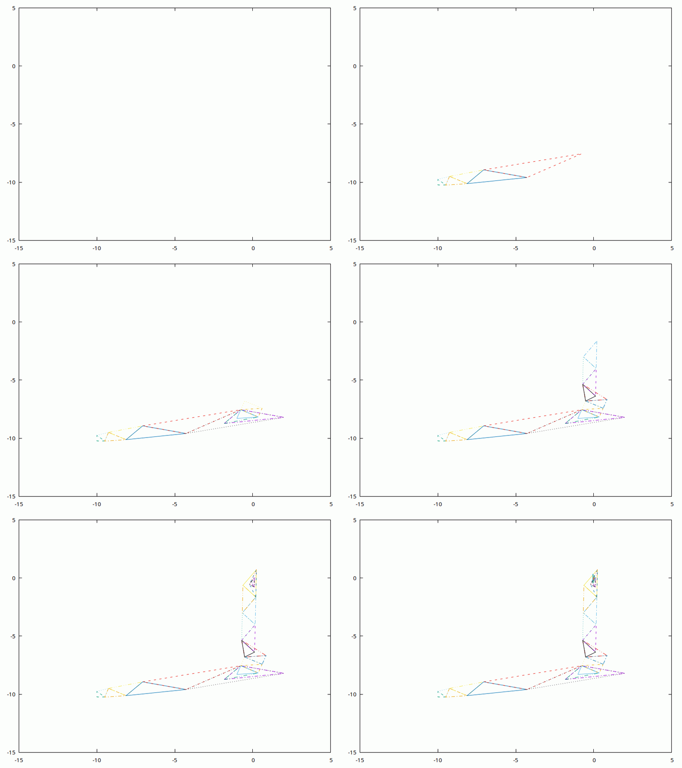
Try a simple ellipsoid; the multiplier makes the algorithm prioritise the first (X) dimension, as you'll see on the plot.

$w->plot(with=>'lines', [0], [1], {xrange=>[-15,5],yrange=>[-15,5]});
my $mult = pdl 4,1;
sub func { (($mult * $_[0]) ** 2)->sumover }
sub logs {
  $w->oplot(with=>'lines', $_[0]->glue(1,$_[0]->slice(",0"))->using(0,1));
}
simplex(pdl(-10,-10), 0.5, 0.01, 30,
  \&func,
  \&logs
);

Now the first of two examples contributed by Alison Offer. These values are for both:

$minsize = 1.e-6; # convergence: if simplex points are this far apart, stop
$maxiter = 100; # max number of iterations: if done these many, stop

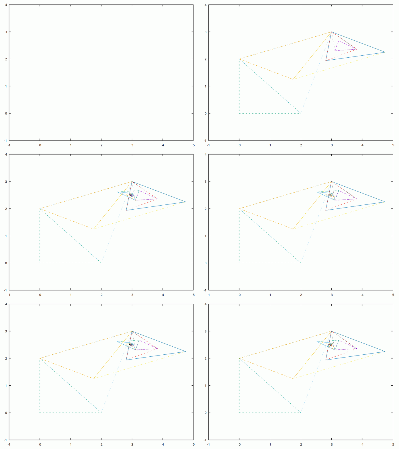
Now we minimise polynomial: (x-3)^2 + 2*(x-3)*(y-2.5) + 3*(y-2.5)^2

$w->plot(with=>'lines', [0], [1], {xrange=>[-1,5],yrange=>[-1,4]}); # reset
$init = pdl [ 0 , 1 ];
$initsize = 2;
($optimum,$ssize,$optval) = simplex($init,$initsize,$minsize,$maxiter,
  sub {
    my ($x, $y) = $_[0]->using(0,1);
    ($x-3)**2 + 2*($x-3)*($y-2.5) + 3*($y-2.5)**2;
  },
  \&logs
);

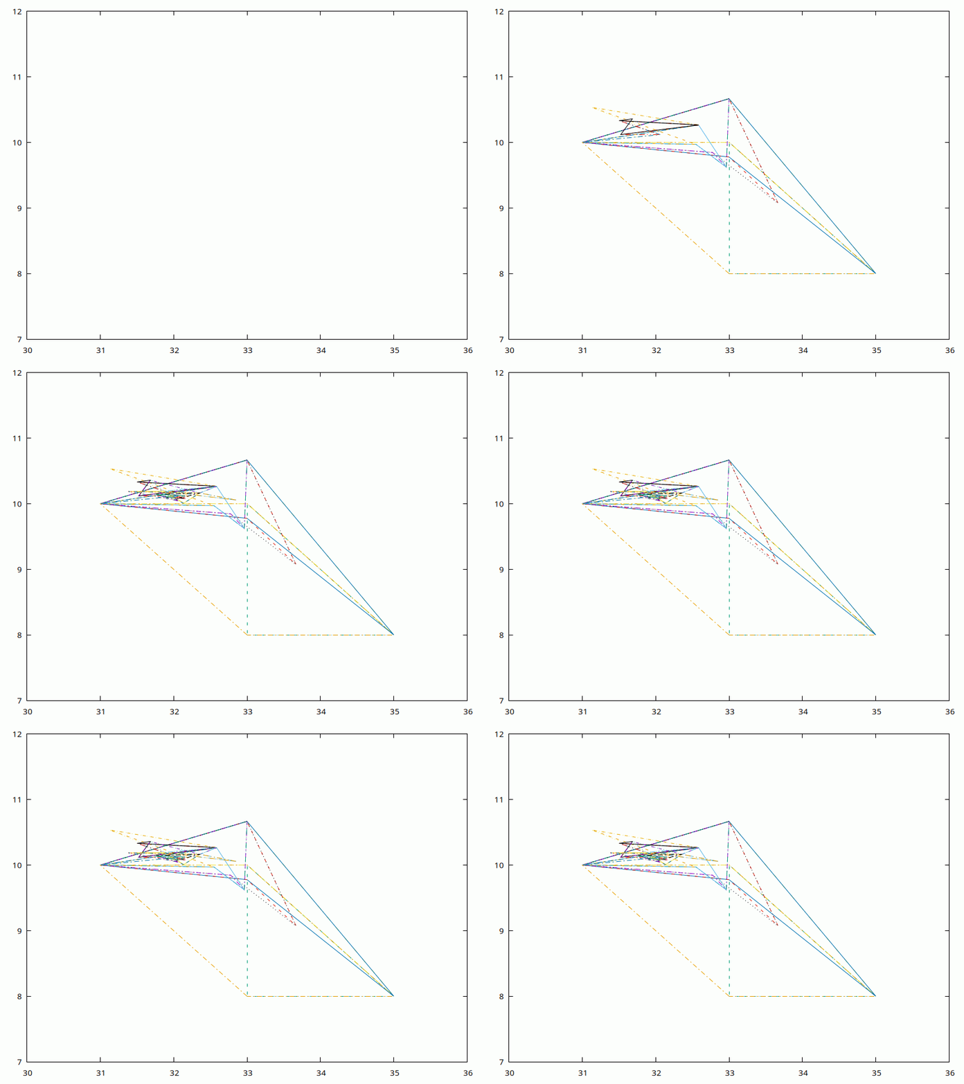
Now to minimise least squares Gaussian fit to data + noise: 32 *exp (-((x-10)/6)^2) + noise

$factor = 3; # noise factor

data : gaussian + noise

$j = sequence(20); srandom(5);
$data = 32*exp(-(($j-10)/6)**2) + $factor * (random(20) - 0.5);
$init = pdl [ 33, 9, 12 ];
$initsize = 2;

The plotting will flatten, i.e. ignore, the third dimension in the vectors.

$w->plot(with=>'lines', [0], [1], {xrange=>[30,36],yrange=>[7,12]}); # reset
($optimum,$ssize,$optval) = simplex($init,$initsize,$minsize,$maxiter,
  sub {
    my ($x, $y, $z) = map $_[0]->slice($_), 0..2;
    (($data - $x*exp(-(($j-$y)/$z)**2))**2)->sumover;
  },
  \&logs
);

Further resources

There are other optimisation modules for PDL, including:

• PDL::Opt::GLPK
• PDL::Opt::NonLinear
• PDL::Opt::QP
• PDL::Opt::ParticleSwarm

Take a look at the Wikipedia page for the simplex algorithm for more on the subject.